Activity 8: Classification predictions and gradients Live

2026-02-24

Imports and data loading

import numpy as np
import pandas as pd
import seaborn as sns
import matplotlib.pyplot as plt
from palmerpenguins import load_penguins
from sklearn.linear_model import LogisticRegression

# Load Palmer Penguins and filter to Adelie vs Chinstrap
df = load_penguins()
penguin_df = df[df["species"].isin(["Adelie", "Chinstrap"])].dropna(subset=["bill_length_mm", "bill_depth_mm"])

# Features: bill_length_mm and bill_depth_mm
X_train = penguin_df[["bill_length_mm", "bill_depth_mm"]].values
feature_names = ["bill_length_mm", "bill_depth_mm"]

# Labels: Adelie = 0, Chinstrap = 1
y_train = (penguin_df["species"] == "Chinstrap").astype(int).values

print(f"Number of examples: {len(y_train)}")
print(f"Number of Adelie (y=0): {np.sum(y_train == 0)}")
print(f"Number of Chinstrap (y=1): {np.sum(y_train == 1)}")
print(f"Feature matrix shape: {X_train.shape}")

penguin_df['y'] = y_train

Number of examples: 219
Number of Adelie (y=0): 151
Number of Chinstrap (y=1): 68
Feature matrix shape: (219, 2)

Part 1: Linear decision boundaries

The above cell loads in our data into penguin_df.

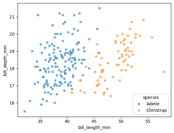
Let’s visualize our two features, colored by species. Let’s create a scatterplot with:

• x="bill_length_mm"

• y="bill_depth_mm"

• hue="species"

• data=penguin_df

• alpha=0.6

sns.scatterplot(
    x="bill_length_mm", 
    y="bill_depth_mm",
    hue="species", 
    data=penguin_df,
    alpha=0.6
)
display(penguin_df.head())

	species	island	bill_length_mm	bill_depth_mm	flipper_length_mm	body_mass_g	sex	year	y
0	Adelie	Torgersen	39.1	18.7	181.0	3750.0	male	2007	0
1	Adelie	Torgersen	39.5	17.4	186.0	3800.0	female	2007	0
2	Adelie	Torgersen	40.3	18.0	195.0	3250.0	female	2007	0
4	Adelie	Torgersen	36.7	19.3	193.0	3450.0	female	2007	0
5	Adelie	Torgersen	39.3	20.6	190.0	3650.0	male	2007	0

Suppose that we have the following weights:

# Weights for a 2D model using bill_length_mm and bill_depth_mm
w0 = -24.5
w1 = 1.35   # weight for bill_length_mm (x1)
w2 = -1.9   # weight for bill_depth_mm (x2)

We can again solve for the decision boundary by setting \(h=0\):

\[0 = w_0 + w_1 x_1 + w_2 x_2\]

\(x_2\) is on the y-axis in our plot, so we can solve for it:

\[ -w_2 x_2 = w_0 + w_1 x_1 \quad \Longrightarrow \quad x_2 = -\frac{w_0 + w_1 x_1}{w_2} \]

Let’s plot this line over our data:

# Two x1 endpoints to draw the boundary line
x1 = np.array([35, 55])


# TODO compute the corresponding x2 values on the decision boundary
x2 = -(w0 + w1*x1) / w2

sns.scatterplot(
    x="bill_length_mm", 
    y="bill_depth_mm",
    hue="species", 
    data=penguin_df,
    alpha=0.6
)
plt.plot(x1, x2, color="black")
plt.ylim(15,22)
#plt.xlim(40, 50)

(15.0, 22.0)

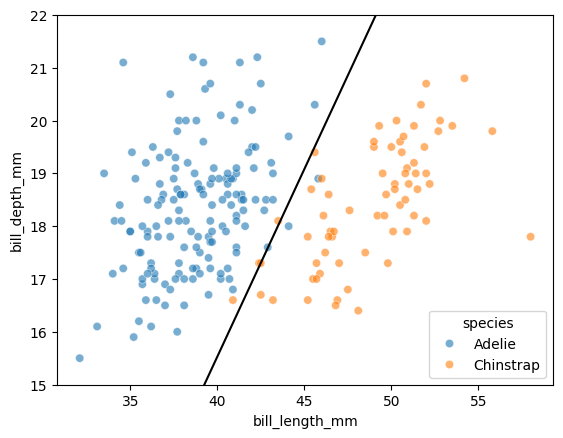
Takeaway

Even though the sigmoid function is non-linear, the decision boundary is going to be linear in the features!

Part 2: Generating probabilities and predictions

LogisticRegression from scikit-learn works the same way as LinearRegression: we call .fit(X, y) to train the model.

# TODO creates a LogisticRegression model and fit it on X and y
model = LogisticRegression()
model.fit(X_train, y_train)

# Print the learned weights
print(f"Intercept (w0): {model.intercept_[0]:.4f}")
print(f"Weights: {model.coef_[0]}")
print(f"  w1 (bill_length): {model.coef_[0][0]:.4f}")
print(f"  w2 (bill_depth):  {model.coef_[0][1]:.4f}")

Intercept (w0): -24.5494
Weights: [ 1.35804435 -1.92413248]
  w1 (bill_length): 1.3580
  w2 (bill_depth):  -1.9241

But unlike LinearRegression, logistic regression can output probabilities using the .predict_proba() method:

This returns an array of shape (n, 2) where:

• Column 0: probability of class 0 (Adelie)

• Column 1: probability of class 1 (Chinstrap)

# TODO: call predict_proba() on the model with input X
proba = model.predict_proba(X_train)

print(f"Shape of proba: {proba.shape}")
print(f"\nFirst 5 rows of proba:")
print(proba[:5])

Shape of proba: (219, 2)

First 5 rows of proba:
[[9.99407822e-01 5.92177979e-04]
 [9.87709002e-01 1.22909979e-02]
 [9.88508221e-01 1.14917793e-02]
 [9.99992825e-01 7.17502671e-06]
 [9.99979912e-01 2.00882817e-05]]

Predictions are then made by picking the class with the highest probability:

# TODO: call predict on the model with input X
preds = model.predict(X_train)

print(f"Shape of preds: {preds.shape}")
print(f"\nFirst 5 rows of preds:")
print(preds[:5])

Shape of preds: (219,)

First 5 rows of preds:
[0 0 0 0 0]

Let’s look at how to compute these outputs on our own.

Suppose we have the \(P(y = 1)\) probabilities from the slides:

proba1_chinstrap = np.array([0.16, 0.78, 0.29, 0.92, 0.52])

print(proba1_chinstrap)
print(proba1_chinstrap.shape)

[0.16 0.78 0.29 0.92 0.52]
(5,)

To convert a 1D array of shape (n,) into a 2D array with shape (n, 1), we can use np.reshape:

# the -1 means "infer the size of the other dimension"
proba1_chinstrap = proba1_chinstrap.reshape(-1, 1)

print(proba1_chinstrap)
print(proba1_chinstrap.shape)

[[0.16]
 [0.78]
 [0.29]
 [0.92]
 [0.52]]
(5, 1)

Since we know that probabilities must sum to 1, what is the line of code that can generate the 2D array for the \(P(y = 0)\) probabilities? Hint: recall what happens when we perform arithmetic between a number and a NumPy array.

Submit the line of code here: https://pollev.com/tliu

# TODO: this can be done in one line!
proba0_adelie = 1 - proba1_chinstrap

print(proba0_adelie)

[[0.84]
 [0.22]
 [0.71]
 [0.08]
 [0.48]]

np.column_stack() then can be used to stack arrays column-wise:

proba_array = np.column_stack([proba0_adelie, proba1_chinstrap])

print(proba_array)

[[0.84 0.16]
 [0.22 0.78]
 [0.71 0.29]
 [0.08 0.92]
 [0.48 0.52]]

How do we then go from this proba_array to a 1D array of predictions?

np.argmax() finds the index of the maximum value, and can be used with axis operations

• axis=1 means: find the index of the maximum value within each row

• axis=0 means: find the index of the maximum value within each column

• no axis means: find the index of the maximum value in the entire array

Note the shape changes:

print(proba_array)
print(proba_array.shape)  # (n, 2)
print("-----------------")

print(np.argmax(proba_array, axis=1))

[[0.84 0.16]
 [0.22 0.78]
 [0.71 0.29]
 [0.08 0.92]
 [0.48 0.52]]
(5, 2)
-----------------
[0 1 0 1 1]

What axis should we use to generate predictions from proba_array?

predictions = np.argmax(proba_array, axis=1)

Part 3: Broadcasting practice

On HW 1, we computed the gradient descent update rule “manually” for each of the weights:

\[\begin{split} w_{1, \text{new}} &= w_{1, \text{old}} - \alpha \frac{\partial \mathcal{L}}{\partial w_1} \\ w_{2, \text{new}} &= w_{2, \text{old}} - \alpha \frac{\partial \mathcal{L}}{\partial w_2} \end{split}\]

Today, we’ll practice using broadcasting to perform a gradient update for all the weights at once.

Suppose we had some loss function \(\mathcal{L}\) such that the gradient with respect to weights \(w_1, w_2, \ldots, w_p\) is given by:

\[ \frac{\partial \mathcal{L}}{\partial w_j} = \sum_{i=1}^n y_i x_{i,j} \]

This gives the gradient update rule for all the weights:

\[ w_{j, \text{new}} = w_{j, \text{old}} - \alpha \sum_{i=1}^n y_i x_{i,j} \]

Given the y’s as a 1D array y of shape (n,), and the data matrix X of shape (n, p), we can compute the gradient update for all the weights at once using broadcasting.

Let’s trace through the broadcasting with a small example (\(n=3\) examples, \(p=2\) features):

# Small example to show broadcasting
X = np.array([[1, 2],
              [2, 4],
              [5, 6]])
y = np.array([1, 0, 1])

print(f"X shape: {X.shape}")
print(X)
print("-----------------")

print(f"y shape: {y.shape}")
print(y)

X shape: (3, 2)
[[1 2]
 [2 4]
 [5 6]]
-----------------
y shape: (3,)
[1 0 1]

Out goal is to compute the summation gradient term for all the weights simultaneously with broadcasting:

\[ \begin{bmatrix} \sum_{i=1}^n y_i x_{i,1} & \sum_{i=1}^n y_i x_{i,2} \end{bmatrix} \]

To do so, we multiply each feature of X by y element-wise:

\[\begin{split} \begin{bmatrix} 1\times1 & 1\times2 \\ 0 \times 2 & 0 \times 4 \\ 1 \times 5 & 1 \times 6 \end{bmatrix} = \begin{bmatrix} 1 & 2 \\ 0 & 0 \\ 5 & 6 \end{bmatrix} \end{split}\]

And then sum over the rows:

\[ \begin{bmatrix} 1 + 0 + 5 & 2 + 0 + 6 \end{bmatrix} = \begin{bmatrix} 6 & 8 \end{bmatrix} \]

In order for y to broadcast with X, we need to reshape y to have shape (3, 1):

# TODO: update y to be 2D with shape (n, 1)
y_reshaped = y.reshape(-1, 1)

print(y_reshaped)
print(y_reshaped.shape)

[[1]
 [0]
 [1]]
(3, 1)

# this will give us a broadcasting error
#y * X

# TODO: use y_shaped to properly broadcast with X
y_reshaped * X

array([[1, 2],
       [0, 0],
       [5, 6]])

Then, we use axis=0 to np.sum over the rows:

# TODO take the sum over the rows, resulting in shape (p,)
# if this array is (n,p)
result = np.sum(y_reshaped * X, axis=0)

print(result)
print(result.shape)

[6 8]
(2,)

result is a 1D array with shape (p,), which can be used to update all the weights at once:

\[\begin{split} w_{1, \text{new}} &= w_{1, \text{old}} - \alpha \underbrace{\sum_{i=1}^n y_i x_{i,1}}_{\text{result[0]}} \\ w_{2, \text{new}} &= w_{2, \text{old}} - \alpha \underbrace{\sum_{i=1}^n y_i x_{i,2}}_{\text{result[1]}} \end{split}\]

w_old = np.array([0, 1])
alpha = 0.1

# TODO: all 2 weights are updated at once without a loop
w_new = w_old - alpha * result

NumPy broadcasting allows this to work for any number of features \(p\), and the gradient update on HW 2 will use this same technique.