HW 1 part 1#
Linear Regression: Foundations
—TODO your name here
Collaboration Statement
TODO brief statement on the nature of your collaboration.
TODO your collaborator’s names here
Part 1 Table of Contents and Rubric#
Section |
Points |
|---|---|
Mathematical Foundations |
2 |
Gradient Descent Implementation |
2.5 |
Total |
4.5 pts |
Notebook and function imports#
import numpy as np
# random number generator
rng = np.random.RandomState(42)
1. Mathematical Foundations [2 pts]#
We’ll begin by deriving the equations that we’ll need to build our linear regression model. Building off what we did in class, linear regression can be expanded to include multiple features.
In particular, if we have a dataset with \(n\) datapoints and \(p\) features, then the linear regression model can be written as:
Where \(\vec{x_i} = (x_{i,1}, x_{i,2}, \ldots, x_{i,p})\) is a vector of features.
We then pair this model with the mean squared error loss function that measures the squared error between the predicted and true values:
The question we now have is: how do we find the “best” values for the weights \(\vec{w} = (w_0, w_1, \ldots, w_p)\) so that the loss function is minimized? To get us started, we’ll need the partial derivatives of the loss function with respect to the weights.
1.1 Linear regression gradients [1 pt]#
Compute the partial derivative of the loss function \(\mathcal{L}(\vec{w})\) with respect to the weight \(w_0\):
Your response:
Now, compute the partial derivative of the loss function with respect to the weight \(w_j\) where \(j \in \{1, 2, 3,\ldots, p\}\):
Your response:
Hint
This derivation should closely follow what we did in class, except now generalized to \(p\) features. Please make an initial attempt on your own but feel free to look at the slides if you get stuck.
Remember that when computing partial derivatives, we treat all variables except the one we are differentiating as constants!
1.2 Gradient descent constant factors [0.5 pts]#
In certain textbooks, you might see the loss function for linear regression written as:
where there is an extra constant factor of \(\frac{1}{2}\) in the loss function. Does multiplying the loss function by a constant factor change which weights are optimal (i.e., minimize the loss)?
To help us answer this question, let’s complete a small derivation. Suppose we have a function \(h(w)\). Let \(w^*\) be the value of \(w\) that minimizes \(h(w)\) over the domain of all real numbers \(\mathbb{R}\). That means for all other values of \(w \in \mathbb{R}\), we have that \(h(w^*) \leq h(w)\). Formally, we can write this as:
Next, let \(g(w) = c \cdot h(w)\), where \(c > 0\) is a constant. Show that \(w^*\) also minimizes \(g(w)\).
Note that this same idea works when the input to the function is a vector of weights \(\vec{w} = (w_0, w_1, \ldots, w_p)\).
Explain what this tells us about the weights that minimize the loss function \(\frac{1}{2n} \sum_{i=1}^n (f(\vec{x}_i) - y_i)^2\) versus the weights that minimize the loss function \(\frac{1}{n} \sum_{i=1}^n (f(\vec{x}_i) - y_i)^2\). Discuss why you think the loss function is sometimes written with the \(\frac{1}{2}\).
Your response: TODO
Discussion questions
Whenever a question asks for a discussion, we are not necessarily looking for a particular answer. However, we are looking for engagement with the material, so one-word/one-phrase answers usually don’t give enough space to show your thought process. Try to explain your reasoning in ~1-2 full sentences.
1.3 Contour plots [0.5 pts]#
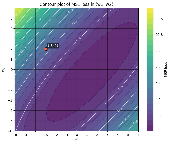
Suppose we’re optimizing the MSE loss function \(\mathcal{L}\) where there are two weights \(w_1\) and \(w_2\). A contour plot using this loss function is shown above. We can think of the partial derivatives \(\frac{\partial \mathcal{L}}{\partial w_1}\) and \(\frac{\partial \mathcal{L}}{\partial w_2}\) as vectors that point in the steepest direction of the loss function.
To get us oriented with this contour plot: the darker the color, the lower the MSE loss, and some of the contour lines are also labelled with the loss value. For example, the labelled point \((w_1, w_2) = (-3, 2)\) sits on the contour with an MSE loss of around 3.
1.3.1: Pick a point on the contour plot that has a higher loss than 3:
The way we think about moving along the contour plot is that increasing or decreasing \(w_1\) corresponds to moving horizontally (left or right) along the contour plot, while increasing or decreasing \(w_2\) corresponds to moving vertically (up or down). Now, consider that the gradient descent algorithm updates the weights by moving in the direction of the negative partial derivatives to minimize the loss function. For example, the update rule for \(w_1\) is given by:
for some learning rate \(\alpha\), and \(w_{1, \text{new}}\) will update such that the overall MSE loss is lower (subject to an appropriately chosen \(\alpha\)).
Now, consider the labelled point \((w_1, w_2) = (-3, 2)\):
1.3.2: Does \(w_1\) need to increase or decrease to move towards the minimum loss?
Your response: TODO
1.3.3: Does \(w_2\) need to increase or decrease to move towards the minimum loss?
Your response: TODO
2. Gradient Descent Implementation [2.5 pts]#
2.1 Gradient update rule [1 pt]#
For the rest of the homework, let’s suppose that \(p=2\), so we have two features \(x_1\) and \(x_2\). Then the linear regression model can be written as:
We can then implement the gradient update rule for the weights. Gradient descent updates the weights by moving in the direction of the negative partial derivatives, scaled by a learning rate \(\alpha\):
Implement this gradient update rule in linreg_grad_update below.
Hint
This function can be written without any loops by using the slice notation for numpy arrays we practiced in Worksheet 1. You can take advantage of numpy’s vectorized operations when computing the predictions for all the data points at once, which is much more efficient than computing the predictions one data point at a time.
For example, X[:, 0] is a 1D numpy array of shape (n,) that contains the first feature of all the data points, and can be multiplied with w_old[1] to compute \(w_1 x_{1}\) for all the data points simultaneously.
def linreg_grad_update(w_old: np.ndarray, X: np.ndarray, y: np.ndarray, alpha: float) -> np.ndarray:
    """Perform a single gradient update for linear regression.

    Args:
        w_old: the old weights of shape (3,)
        X: the feature matrix of shape (n, 2)
        y: the target vector of shape (n,)
        alpha: the learning rate

    Returns:
        The new weights of shape (3,)
    """

    assert w_old.shape == (3,)

    # TODO your code here
    return None
Tip
The simple test cases we provide via assert statements here usually have data that can be verified by hand if you would like to double check your implementation.
You are encouraged to write your own test cases as well! If you do write additional test cases, just be sure that the assert statements are written within the if __name__ == "__main__": block so that the autograder can run correctly.
if __name__ == "__main__":
    # Initialize some simple data for testing, n=3, p=2
    X = np.array([[1, 2],
                  [2, 3],
                  [3, 3]])
    y = np.array([0, 1, 2])
    w_old = np.array([0, 0, 0])
    alpha = 0.5

    # Test the gradient update rule
    w_new = linreg_grad_update(w_old, X, y, alpha)
    assert w_new.shape == (3,), "The new weights should have shape (3,)"
    assert np.allclose(w_new, np.array([1, 8/3, 3])), "The new weights should be [1, 8/3, 3]"
Gradient notation
As an aside, gradient update rule can be more compactly written in terms of the gradient \(\nabla \mathcal{L}(\vec{w})\), which is the vector of partial derivatives:
The gradient update rule is then given by:
Where \(\vec{w}_{\text{new}}\) and \(\vec{w}_{\text{old}}\) are vectors of shape (3,) holding the new and old weights, respectively. We will discuss this representation in more detail in upcoming classes.
2.2 MSE loss [0.5 pts]#
Now, let’s implement the loss function. Recall from class that the loss function quantifies the amount of error that our model makes on the training data. Thus, our goal is to build a model that minimizes the loss function. From above, the loss function is given by:
Our model \(f(\vec{x}_i)\) outputs predictions \(\hat{y}_i\), giving the loss function as:
def mse_loss(y_hat: np.ndarray, y: np.ndarray) -> float:
    """Compute the mean squared error loss for linear regression.

    Args:
        y_hat: the predicted values of shape (n,)
        y: the target values of shape (n,)

    Returns:
        The mean squared error loss
    """
    assert y_hat.shape == y.shape, "y-hat predictions and y targets must have the same shape"

    # TODO your code here
    return None
if __name__ == "__main__":
    # Test the loss function
    y_hat = np.array([0, 1, 2])
    y = np.array([0, 1, 2])
    assert np.allclose(mse_loss(y_hat, y), 0), "The loss should be 0"

    y_hat = np.array([1, 2, 4])
    y = np.array([0, 1, 2])
    assert np.allclose(mse_loss(y_hat, y), 2), "The loss should be 2"
2.3 Gradient descent [1 pt]#
We’ll now implement the overall gradient descent algorithm. The algorithm begins by initializing the weights to arbitrary values, and then iteratively updates the weights until a stopping criterion is met. There are two stopping criteria:
We stop if the weights have sufficiently converged to a minimum. Here, we test for convergence by checking if the Euclidean distance between the old and new weights is less than some small stopping threshold \(\epsilon\):
We also stop if the number of iterations exceeds a maximum number of iterations.
The algorithm can be described in the following pseudocode:
# Initialize the weights to arbitrary values
w_new = [1e4, 1e4, 1e4]
w_old = np.random.randn(3)
while True:
    # update the new weights
    w_new = linreg_grad_update(w_old, X, y, alpha)

    # check for convergence using Euclidean distance from Worksheet 1, exit the while loop if the weights have converged

    # check if number of iterations exceeds max_iters, exit the while loop if it does

    # update the old weights
    w_old = w_new
In addition to finding the final weights, your implementation will also return a list of the loss values and a list of the weights, appended at each iteration.
Tip
In Python, you can use the break statement to exit the while loop early.
def linreg_grad_descent(X: np.ndarray, y: np.ndarray, alpha: float, stopping_threshold: float=1e-6, max_iters: int=10000) -> tuple[np.ndarray, list[float], list[np.ndarray]]:
    """Perform gradient descent for linear regression.

    Additionally computes the loss function at each iteration.

    Args:
        X: the feature matrix of shape (n, 2)
        y: the target vector of shape (n,)
        alpha: the learning rate
        stopping_threshold: the stopping threshold, default is 1e-6
        max_iters: the maximum number of iterations, default is 10000

    Returns:
        Final weights of shape (3,)
        A list of the loss function values at each iteration
        A list of the weights at each iteration
    """

    # Initialize the weights to arbitrary values
    w_new = [1e4, 1e4, 1e4]
    w_old = np.random.randn(3)

    # Initialize the loss values list
    loss_values = []

    # Initialize the weight history list
    w_history = []

    # number of iterations
    num_iters = 0

    # TODO Complete the while loop
    while True:
        # Compute the loss function using the old weights


        # Append to the loss values list


        # Append the weights to the history


        # Update the new weights


        # Check for convergence by seeing if the Euclidean distance between the
        # old and new weights is less than the stopping threshold, exit the loop if so


        # Check if number of iterations exceeds max_iters, exit the loop if so


        # Update the old weights


        # Increment the number of iterations
        num_iters += 1


    return w_new, loss_values, w_history
if __name__ == "__main__":
    # Initialize some simple data for testing, n=3, p=2
    X = np.array([[1, 2],
                  [2, 3],
                  [3, 3]])
    y = np.array([0, 1, 2])
    alpha = 0.05

    # Test the gradient descent algorithm
    w_final, loss_values, w_history = linreg_grad_descent(X, y, alpha)

    assert w_final.shape == (3,), "The final weights should have shape (3,)"
    assert loss_values[-1] < 1e-4, "The final loss should be less than 1e-4"
    assert np.allclose(w_final, np.array([-1, 1, 0]), atol=1e-3), "The final weights should be [-1, 1, 0]"
How to submit
Like Worksheet 1, follow the instructions on the course website to submit your work. For part 1, you will submit hw1_foundations.ipynb and hw1_foundations.py.