Worksheet 1#
Getting Started
—TODO your name here
Collaboration Statement
TODO brief statement on the nature of your collaboration.
TODO your collaborator’s names here.
Learning Objectives#
Get familiarized with the Jupyterhub interface and the course’s submission system.
Practice with the first math concepts needed for the course:
Derivatives
Vectors
Norms and distances
Practice with
numpyarray usage.Learn about OOP concepts in Python with
sklearn.
1. Course resources [0.5 pts]#
1.1: Read through all the pages listed in the syllabus section on the course website. What are the two file types that you need to submit to Gradescope for each assignment?
Your Response: TODO
1.2 Reply to the Course Intros thread on Ed introducing yourself and sharing why you’re interested in taking this course.
TODO post to the Ed discussion thread: https://edstem.org/us/courses/94030/discussion/7575488
Coding interface#
Programming language: Python. This course will be taught in Python. To get the most out of the course, it’s important you don’t feel bogged down by the syntax of the language so that you can focus on the concepts introduced. If you do not have prior experience with Python, that’s no problem. Please do take the time at start of the course to study and practice it.
For resources, I recommend going through an online Python tutorial such as this one: https://www.learnpython.org/, and completing all the sections under “Learn the Basics.”
Libraries. We will be using a standard Python machine learning stack throughout the course:
sklearn: for building (non-neural network) machine learning models and pipelines
pandas: for data table manipulation and analysis
seaborn + matplotlib: for figure visualization
ipywidgets: for interactive widgets
pytorch: for building and training deep learning models
autograd: for automatic differentiation (more on this later in the semester!)
We will introduce the functionality of these libraries as we need them in the course, so we do not assume prior knowledge of these libraries. However, I do encourage you to refer to the documentation for all of them.
Computing environment. We will be using Jupyter notebooks (.ipynb files) for all assignments. We have a centralized Jupyterhub server which provides a uniform environment for everyone, and you can access it anywhere on campus using your MHC credentials:
Warning
If you would like to run your code locally, you are welcome to do so and we can provide the necessary list of installation packages. However, note that the teaching team unfortunately cannot help troubleshoot issues with your local environment. In particular, some of the scientific computing libraries can be finnicky to install on ARM-based Macs, which is why we have centralized our Jupyterhub server.
There are two types of cells in a Jupyter notebook:
Code cells: for writing and running code
Markdown cells: for writing text
1.3 TODO Create a new code cell below that defines a function called hello() that takes no arguments and returns the string "Hello, COMSC 335!"
Tip
Many of the functions we ask you to implement in the course will be autograded. There will be no submission limit, so feel free to submit multiple times to get feedback on your work!
We will frequently provide some simple test cases via assert statements wrapped in a if __name__ == "__main__": block to check your function, like the one below. The syntax for assert statements is as follows:
assert bool_expression, description
where the bool_expression is a boolean expression that tests some condition, and the description is a string that will be displayed if the assertion fails (evaluates to False).
You are encouraged to write your own test cases as well for your functions!
if __name__ == "__main__":
    # check that hello() returns the specified string
    assert hello() == "Hello, COMSC 335!", "hello() does not return the correct string"
Jupyter notebooks allow users to write code and text in the same file. The language used to write text is called Markdown, and is popular language for writing documentation (for example, Github README files default to Markdown).
In particular, Markdown allows users to write mathematical notation using LaTeX. Read through this guide to learn how to format markdown cells with LateX, as you will be typesetting some mathematical statements in the assignments.
Tip
If you double click on a cell with a math equation, you can view the LaTeX source code for the cell that you can copy and paste into your own markdown cells.
Math#
We will be using mathematical notation to formalize many concepts in this course. For example, the notation for sums is as follows:
which can be read as “the sum of \(x_i\)’s from \(i=1\) to \(n\)”.
You may also see only a subscript underneath the summation symbol, which means the sum is over all the elements in the set. For example, the sum of all elements in the set \(A=\{1,2,3\}\) is written as:
2. Calculus primer [1 pt]#
In this course, we will be making frequent use of derivatives for optimization. Recall from your calculus classes that the derivative of a function \(f(x)\) points in the direction of steepest ascent of the function. The derivative is sometimes denoted as \(f'(x)\) or \(\frac{d}{dx} f(x)\). Here, will use the latter notation to more closely align with the notation used for partial derivatives of functions with multiple inputs.
Here is a list of some common differentiation rules that will be useful when brushing up on calculus:
Common Differentiation Rules
Constant multiple rule:
Constant rule:
Sum rule:
Product rule:
Quotient rule:
Chain rule:
2.1: What is the derivative of \(f(x) = 3x^2 + 2x + 5\)? Typeset your answer in LaTeX below.
2.2: Using the chain rule, what is the derivative of \(h(x) = (2x + 1)^3\)? Typeset your answer in LaTeX below.
Solutions (click this to check once you’ve completed 2.1 and 2.2)
2.1:
2.2:
Partial derivatives#
Most machine learning models are functions of multiple variables. Thus, we need to extend the concept of derivatives to multiple variables, which are called partial derivatives.
We find partial derivatives by varying one variable at a time, holding all of the other variables constant. For example, the partial derivative of a function \(f(x_1, x_2)\) with respect to \(x_1\) is found by treating \(x_2\) as a constant and differentiating with \(x_1\) as the variable of interest. This is denoted as:
In general, we treat all variables except the one we are differentiating with respect to as constants.
For example, suppose we have a function \(f(x_1, x_2) = (x_1 + 2x_2^3)^2\). Then, the partial derivative of \(f\) with respect to \(x_1\) is:
2.3: Compute the partial derivative of \(f(x_1, x_2) = (x_1 + 2x_2^3)^2\) with respect to \(x_2\).
We may also encounter taking partial derivatives of functions over sums. For example, consider the following function:
We might want to compute the partial derivative of \(f\) with respect to some \(x_q\) where \(q \in \{1, 2, \ldots, p\}\):
While this might look a little daunting, we can apply the rules shown so far to compute the partial derivatives. Let’s do this step by step.
First, we can split the summation into \(p\) terms:
Then, by the sum rule and the fact that all other variables are treated as constants, we can compute the partial derivative of \(f\) with respect to \(x_q\) as follows:
2.4: Consider the following function of five variables, \((w_1, w_2, w_3, w_4, w_5)\):
Compute the partial derivative of \(f\) with respect to \(w_3\).
Solutions (click this to check once you’ve completed 2.3 and 2.4)
2.3:
2.4:
3. NumPy fundamentals [2 pts]#
NumPy Arrays#
NumPy is the standard Python library for scientific computing. The standard import idiom for the library is as follows:
# the standard way to import numpy
import numpy as np
We can then use the np prefix to access the functions and classes in the library. The primary data structure in NumPy is the ndarray, which is a multi-dimensional array of elements of the same type, typically integers or floats.
We can create an ndarray using the np.array() function and passing in Python lists. For example:
import numpy as np

a = np.array([1, 2, 3, 4]) # create an array from a list
print(type(a)) # Will print <class 'numpy.ndarray'>
print(a) # pretty prints the array
A fundamental property of a NumPy array is its shape, which is a tuple of integers that represent the size of the array in each dimension. For example, the shape of the array a is (4,), which means it has 4 elements in one dimension:
print(a.shape) # Will print (4,)
We can thus create two-dimensional arrays by passing in a list of lists to the np.array() function:
# creates 2-row, 3-column array with a list of lists
b = np.array([[1, 2, 3], [4, 5, 6]])

# the same array, but formatted for better readability
b = np.array([[1, 2, 3],
              [4, 5, 6]])

# prints the array
print(b.shape)
The shape of b is (2, 3), which means it has 2 rows and 3 columns.
The shape tuple itself provides useful information about the array and can be accessed using [ ] notation:
# prints the first element of the shape tuple, which is the number of rows in b
print(b.shape[0])

# prints the second element of the shape tuple, which is the number of columns in b
print(b.shape[1])
3.1 Complete the function below to create an array of shape (4, 2) with any values you want in it.
Python Return Type Hints
You’ll notice that the function definition includes -> np.ndarray. This is a Python type hint that indicates the function returns an np.ndarray. These hints are not required for Python code to run, but is good practice to include in order to increase the readability of your code. They are also used by some text editors like VSCode to provide type-checking and documentation. Most of the functions you will see in this course will have type hints.
def shape_practice() -> np.ndarray:
    """Practice with creating arrays of a specific shape.

    Returns:
        A 2D array of shape (4, 2)
    """

    # TODO your code here
    return None
if __name__ == "__main__":
    result = shape_practice()
    assert result.shape == (4, 2), "result should be a 2D array of shape (4, 2)"
There are helper functions that can be used to create arrays with specific values:
zeros = np.zeros((2, 3)) # create a shape (2, 3) array with all elements equal to 0
print(zeros)
print("----")
ones = np.ones((4, 4)) # create a shape (4, 4) array with all elements equal to 1
print(ones)
Indexing and Slicing#
NumPy arrays can be indexed in a variety of different ways. To begin, we can access elements using square brackets. For example, we can access index 0 of a as follows:
# Show the whole array
print(a)

# NumPy arrays are 0-indexed
print(a[0]) # Will print 1
Just like with Python lists, we can use negative indices to access elements from the end of the array. For example, a[-1] will return the last element of a:
print(a[-1]) # Will print 4
If the array is multidimensional, we can access elements by specifying the index for each dimension. For example, we can access the element in the second row and third column of b as follows:
# Show the whole array
print(b)

# Access the element in the second row and third column
print(b[1, 2]) # Will print 6
NumPy arrays also support slicing with the colon : operator, which allows us to access a range of elements in the array. If a : is used as the index, it is interpreted as “take all elements in this dimension”:
# Show the whole array
print(b)

# Access the first row
print(b[0, :]) # Will print [1 2 3]

# Access the second column. Note that the selection is a 1D array so there no notion of a "column vector" in NumPy
print(b[:, 1]) # Will print [2 5]
The slice operator can be combined with beginning and ending indices to access a range of elements:
# Show the whole array
print(b)

print("----")
# Access the first two columns of row 0
print(b[0, :2]) # Will print [1 2]
print("shape of b[0, :2]:", b[0, :2].shape)
print("----")

# Access all rows and the last two columns
print(b[:, 1:]) # Will print [[2, 3],
#                             [5, 6]]
print("shape of b[:, 1:]:", b[:, 1:].shape)
print("----")
We need to pay attention to the shape of the array when slicing. Note how the first selection above returns a 1D array of shape (2,), while the second selection returns a 2D array of shape (2, 2).
3.2: Consider the array c defined in the function below. Use indexing to access [4, 6] from c and return it.
def index_practice() -> np.ndarray:
    """Practice with indexing"""

    c = np.array([[1, 3, 5],
                  [2, 4, 6],
                  [3, 5, 7]])

    # TODO your code here
    return None


if __name__ == "__main__":
    result = index_practice()
    assert result.shape == (2,), "result should be a 1D array of shape (2,)"
    # np.allclose() checks if all elements in the array are equal to the corresponding elements in the other array
    assert np.allclose(result, np.array([4, 6])), "result should be [4, 6]"
3.3: Complete the function below that selects the last column of the passed in array.
Python Parameter Type Hints
You’ll notice that function parameter name is written as arr: np.ndarray. Similar to the return type hint, this is a Python parameter type hint that indicates the function parameter arr is an np.ndarray. Again, these hints are optional and do not affect the execution of the code, but is good practice to include in order to increase the readability of Python code.
def select_last_column(arr: np.ndarray) -> np.ndarray:
    """Select the last column of the passed in array.

    Args:
        arr: A 2D array

    Returns:
        A 1D array of the last column of the passed in array
    """

    # TODO your code here
    return None
if __name__ == "__main__":
    test_arr = np.array([[1, 2],
                         [4, 5]])

    result = select_last_column(test_arr)
    assert np.allclose(result, np.array([2, 5])), "result should be [2, 5]"
Boolean indexing#
We can also apply boolean operators to arrays. These operations return an array of the same shape as the original array, with elements set to True or False depending on the result of the boolean operation. For example, we can check which elements of a are greater than 2:
a = np.array([1, 2, 3, 4])
print(a > 2) # Will print [False False  True  True]
We can then use these boolean arrays to index into the original array:
# Selects the elements of a that are greater than 2
print(a[a > 2]) # Will print [3 4]
3.4: Complete the function below that selects all elements of the passed in array that are even.
def select_evens(arr: np.ndarray) -> np.ndarray:
    """Select all elements of the passed in array that are even.

    Args:
        arr: A 1D array

    Returns:
        A 1D array of the elements of the passed in array that are even.
    """

    # TODO your code here
    return None
if __name__ == "__main__":
    test_arr = np.array([1, 2, 3, 4, 5, 6])
    result = select_evens(test_arr)
    assert np.allclose(result, np.array([2, 4, 6])), "result should be [2, 4, 6]"
Array arithmetic#
Basic arithmetic operations are applied element-wise to arrays. That means that the shapes of the arrays must be the same.
The following code adds two arrays element-wise:
a = np.array([1, 1, 1])
b = np.array([2, 4, 6])

print(a + b) # Will print [3 5 7]
We can also apply arithmetic operations to arrays with scalars (a single number). The scalar is applied to each element in the array:
b = np.array([2, 4, 6])

print(b * 2) # Will print [4 8 12]
3.5 Work out what the following code will print before checking your answer.
a = np.array([2, 1])
b = np.array([-1, 1])

print((a * b) - 1)
Your Response: [TODO]
Solutions (click this to check once you’ve completed 3.5)
The multiplication is also performed element-wise, so we get:
[(2*-1) - 1, (1*1) - 1] = [-3, 0]
Note that this is not the same as matrix multiplication or a dot product. We will cover matrix manipulation and NumPy broadcasting concepts in a future worksheet.
4. Vectors, norms, and distances [1 pt]#
As we’ve seen, machine learning models are functions of potentially many features. Instead of writing out the individual variables (e.g. \(x_1, x_2, \ldots, x_p\)), we can collect them into a vector to represent them. They are often denoted as a bold-faced letter \(\mathbf{x}\) or with an arrow above the letter \(\vec{x}\). In this course, we will use the arrow notation to visually differentiate the vectors from scalars:
These vectors generalize the geometric vectors you might have seen in math courses to higher dimensions. Mapping onto the NumPy concepts we just practiced, we can think of vectors as 1D arrays of shape (p,), where p is the number of elements (and thus the dimensionality) in the vector.
# represents a vector in 3-dimensional space
a = np.array([1, 2, 3])
Norms#
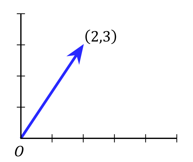
Geometric vectors can be visualized as a line segment in space that starts at the origin. For example, we can represent the two-dimensional vector \(\vec{x} = (2, 3)\) as follows:
We can generalize this notion of length to vectors in any number of dimensions, as well as different ways to measure the “length” of a vector, which is called a norm. Norms are represented using double vertical bars e.g. \(\|\vec{x}\|\), and always produce a scalar value that represents vector length. A commonly used norm is the Euclidean norm, which is defined as:
Euclidean norm
This is also known as the L2 norm (note the 2 in the subscript).
One straightforward way to implement this is to use a for loop for the summation:
def euclidean_norm_slow(x: np.ndarray) -> float:
    """Compute the Euclidean norm of a vector using a for loop.

    Args:
        x: A 1D array

    Returns:
        The Euclidean norm of the vector
    """
    sum = 0
    for i in range(x.shape[0]):
        sum += x[i]**2

    # Computes the square root of the sum
    return np.sqrt(sum)
However, loops are slow in Python for large inputs. NumPy provides many vectorized operations, which can be directly applied to arrays and are highly optimized for performance. Here, let’s use the np.sum() function, which computes the sum of all elements in an array in a single operation:
a = np.array([1, 2, 3])
print(np.sum(a)) # Will print 6
4.1 Complete the function below that computes the Euclidean norm of a vector, replacing the for-loop with np.sum(). You should be able to do this in a single line of code!
def euclidean_norm_vectorized(x: np.ndarray) -> float:
    """Compute the Euclidean norm of a vector *without* using a for loop.

    Args:
        x: A 1D array

    Returns:
        The Euclidean norm of the vector
    """

    # TODO your code here
    return None
if __name__ == "__main__":
    x = np.array([2, 3])

    assert np.allclose(euclidean_norm_vectorized(x), euclidean_norm_slow(x)), "result should be the same as the slow version"
    assert np.allclose(euclidean_norm_vectorized(x), np.sqrt(2**2 + 3**2)), "result should be the same as manual computation"
Timing operations#
Jupyter notebooks also provide a way to measure the time it takes to run a cell of code through a “magic” command (no, really, that’s what they’re actually called), which are generally prefixed with a %. We can use the magic command %timeit to compare the performance of our two implementations, which provides an estimate of the average runtime over multiple runs.
4.2 Use the cell below to time the performance of the two implementations. Approximately how many times faster is the vectorized version?
Your Response:
average runtime of
euclidean_norm_slow(x): TODOaverage runtime of
euclidean_norm_vectorized(x): TODOspeedup: TODO
if __name__ == "__main__":
    # generate a large, random vector with a million elements
    x = np.random.randn(1000000)

    # TODO run the slow version to time it, then the vectorized version
    %timeit euclidean_norm_slow(x)
Takeaway (click this once you’ve completed 4.2)
The exact numbers might vary (and double check the seconds units), but you should see a ~200-400x speedup with the vectorized version!
Whenever possible, we should try to use vectorized operations instead of for-loops when manipulating NumPy arrays – though for-loops are still sometimes necessary.
Distances#
Finally, we can also use norms to measure the distance \(d\) between two vectors. A common distance metric is the Euclidean distance, which is just the Euclidean norm of the difference between two vectors:
4.3 Using your euclidean_norm_vectorized function, complete the function below that computes the Euclidean distance between two vectors:
def euclidean_distance(x: np.ndarray, z: np.ndarray) -> float:
    """Compute the Euclidean distance between two vectors of the same dimensionality.

    Args:
        x: A 1D array, same shape as z
        z: A 1D array, same shape as x

    Returns:
        The distance between the two vectors
    """

    assert x.shape == z.shape, "x and z must have the same shape"

    # TODO your code here
    return None

if __name__ == "__main__":
    x = np.array([1, 2, 3])
    z = np.array([4, 5, 6])
    assert np.allclose(euclidean_distance(x, z), np.sqrt((1-4)**2 + (2-5)**2 + (3-6)**2)), "result should be the same as manual computation"
4.4 Is the Euclidean distance metric symmetric? That is, does \(d(\vec{x}, \vec{z}) = d(\vec{z}, \vec{x})\)?
Your Response: TODO
Solution (click this to check once you’ve completed 4.4)
The Euclidean distance metric is symmetric – notice how the square term in the definition of the Euclidean distance is the same regardless of which point we subtract from which:
5. OOP in Python with sklearn [1 pt]#
Our final topic for this worksheet is a brief introduction to object-oriented programming (OOP) in Python, which we’ll explore using the sklearn library. sklearn is the primary Python library for building (non-deep learning) machine learning models, and is a great example of how OOP is used in practice. Each machine learning model in sklearn is represented as a class, which contains the model’s parameters at initailization, as well as functions for training and predicting.
Let’s walk through and complete the implementation of the k nearest neighbors (KNN) regressor model that we discussed in class.
Class definition#
Classes in Python are defined using the class keyword.
sklearn provides a BaseEstimator class that provides a standard interface for all models, and can be subclassed to create new models. To extend a class, the child class just passes in the parent class name as an “argument” to the class keyword:
# Our KNNRegressor class extends the BaseEstimator class
class KNNRegressor(BaseEstimator):
    ...
Constructor#
In Python, the constructor is defined using the __init__ method. This method is called when a new instance of the class is created. The first argument to the constructor is always self, which refers to the instance of the class itself – think of it as similar to the this keyword in Java.
Any additional arguments to the constructor are passed in by the user when the class is instantiated, and instance variables are also assigned using the self keyword.
# Our KNNRegressor class extends the BaseEstimator class
class KNNRegressor(BaseEstimator):
    """KNN regressor model."""

    def __init__(self, n_neighbors: int):
        """Initializes our KNNRegressor model.

        Args:
            n_neighbors: the number of neighbors to use for the KNN regressor
        """

        # self.var_name is an instance variable that can be accessed by any method in the class
        self.n_neighbors = n_neighbors
Object creation#
Objects are created using the class_name(arguments) syntax. This should look similar to other OOP languages you may have used. For example, we can create a new KNNRegressor object with 5 neighbors as follows:
# Create a new KNNRegressor object with 5 neighbors
knn_model = KNNRegressor(n_neighbors=5)
Note that the self argument is not passed in. It is implicitly passed in by Python when the object is created.
Instance methods#
Instance methods are defined using the def keyword within the class block, and are similar to functions in Python. Like the constructor, the first argument to any instance method is required to be self.
In order for our KNNRegressor class to be a valid sklearn estimator, we need to implement the fit and predict methods:
class KNNRegressor(BaseEstimator):
    ...

    def fit(self, X: np.ndarray, y: np.ndarray) -> Self:
        """Fits the KNN regressor to the training data.

        Note that KNN models do not have any functions or features that need to be fit,
        so all this method does is store the training data in the instance variables.

        Args:
            X: the feature matrix of shape (n, p)
            y: the target vector of shape (n,)

        Returns:
            self: the fitted model
        """

        # Use self to store the training data in the instance variables
        self.X_ = X
        self.y_ = y

        # sklearn fit() methods return the model itself to allow for method chaining
        return self
sklearn uses a convention where any instance variables that are created during the model fitting process are suffixed with a _ (e.g. self.X_). This is actually used by sklearn to determine whether a model has been fitted or not. Another convention is that sklearn fit() methods return the model itself to allow for method calls to be chained together, e.g. knn_model.fit(X_train, y_train).predict(X_new).
Recall from class that the KNN regressor predicts the \(y\) value of a new point by averaging the \(y\) values of the k nearest neighbors. If \(D_k = \{(\vec{x_1}, y_1), (\vec{x_2}, y_2), \ldots, (\vec{x_k}, y_k)\}\) is the set of \(k\) nearest neighbors to a new point \(\vec{x}_{\text{new}}\), then the prediction is given by:
Let’s first write a helper function, find_k_nearest_indices, that finds the indices of the k nearest neighbors to a new point \(\vec{x}\) using the Euclidean distance.
The function is partially implemented below. You will need to use the np.argsort function, which returns the indices that would sort an array. For example, if we wanted to sort the array a = np.array([3, 2, 1]), then np.argsort(a) returns [2, 1, 0], which are the indices that would sort a in ascending order:
a = np.array([3, 2, 1])
print(np.argsort(a)) # Will print [2 1 0]
print(a[np.argsort(a)]) # Will print in sorted order: [1 2 3]
5.1: Complete the function below that implements the logic described above. Hint: You should use the indexing and slice notation from the NumPy section to select each point in X_train, as well as to return the first k elements of the sorted array.
def find_k_nearest_indices(x: np.ndarray, X_train: np.ndarray, k: int) -> list:
    """Finds the indices of the k nearest neighbors to a new point x.

    Args:
        x: the new point of shape (p,)
        X_train: the training data of shape (n, p)
        k: the number of nearest neighbors to find

    Returns:
        the indices of the k nearest neighbors to x in X_train
    """

    dists = []

    for i in range(X_train.shape[0]):
        # TODO append the Euclidean distance between x and the i-th point in X
        dists.append(None)

    # TODO call np.argsort on dists, then return the first k elements
    return None
if __name__ == "__main__":
    # initialize some simple data for testing
    X_train = np.array([[1],
                        [4],
                        [6],
                        [9]])

    # test the find_k_nearest_indices function in one dimension
    x = np.array([7]) # closest two points to 7 are 6 and 9
    k_nearest_indices = find_k_nearest_indices(x=x, X_train=X_train, k=2)

    assert np.allclose(k_nearest_indices, np.array([2, 3])), "result should be the indices of 6 and 9, which are [2,3]"

    # Initialize some two dimensional data for testing
    X_train = np.array([[1, 2],
                        [2, 3],
                        [3, 3]])

    x = np.array([0, 0]) # closest two points to (0,0) are (1,2) and (2,3)
    k_nearest_indices = find_k_nearest_indices(x=x, X_train=X_train, k=2)

    assert np.allclose(k_nearest_indices, np.array([0, 1])), "result should be the indices of (1,2) and (2,3), which are [0,1]"
5.2: Now, let’s put things together. The KNNRegressor class is given below, and your job is to complete the predict method using the helper function you just implemented:
from sklearn.base import BaseEstimator
from typing import Self

# Our KNNRegressor class extends the BaseEstimator class
class KNNRegressor(BaseEstimator):
    """KNN regressor model."""


    def __init__(self, n_neighbors: int):
        """Initializes the KNN regressor model.

        Args:
            n_neighbors: the number of neighbors to use for the KNN regressor
        """

        # self.var_name is an instance variable that can be accessed by any method in the class
        self.n_neighbors = n_neighbors


    def fit(self, X: np.ndarray, y: np.ndarray) -> Self:
        """Fits the KNN regressor to the training data.

        Note that KNN models do not have any functions or features that need to be fit,
        so all this method does is store the training data as instance variables.

        Args:
            X: the data examples of shape (n, p)
            y: the answers vector of shape (n,)

        Returns:
            self: the fitted model
        """

        # Use self to store the training data in the instance variables
        self.X_ = X
        self.y_ = y

        # As convention, sklearn fit() methods return the model itself to allow for method chaining
        return self


    def predict(self, X: np.ndarray) -> np.ndarray:
        """Predicts the values of a set of new points X.

        Args:
            X: the new points of shape (n_new, p)

        Returns:
            the predicted values of shape (n_new,)
        """

        assert self.X_.shape[1] == X.shape[1], "X must have the same number of features as the training data"

        predictions = []

        # this loops over the rows of X
        for x in X:
            # TODO find the k nearest neighbors to x


            # TODO compute the average of the k nearest neighbors, append to predictions
            predictions.append(None)

        return np.array(predictions)
if __name__ == "__main__":
    # initialize some simple data for testing
    X_train = np.array([[1],
                        [4],
                        [6],
                        [9]])

    y_train = np.array([1, 2, 3, 4])

    # test the predict method
    knn_model = KNNRegressor(n_neighbors=2)
    knn_model.fit(X_train, y_train)

    x = np.array([[7]]) # note that x is a 2D array of shape (1, 1)!
    assert np.allclose(knn_model.predict(x), 3.5), "result should be (3 + 4) / 2 = 3.5"

    # Initialize some two dimensional data for testing
    X_train = np.array([[1, 2],
                        [2, 3],
                        [3, 3]])

    y_train = np.array([1, 2, 3])
    X_new = np.array([[0, 0],  # closest two points to (0,0) are (1,2) and (2,3)
                  [5, 5]]) # closest two points to (5,5) are (3,3) and (2,3)

    knn_model = KNNRegressor(n_neighbors=2)
    knn_model.fit(X_train, y_train)
    assert np.allclose(knn_model.predict(X_new), np.array([1.5, 2.5])), "result should be (1 + 2) / 2 = 1.5 and (3 + 2) / 2 = 2.5"
n_neighbors and model “complexity”#
We will frequently use interactive widgets to explore tradeoffs in building machine learning models. We will cover how to implement these widgets in a future worksheet, but for now, the code to run the widget will be provided.
We will consider a simple prediction task, where our goal is to predict block-level housing prices based on a single feature: the median income of the block:
\(X\) is an
(n, 1)array of median incomes on a block, measured in tens of thousands of dollars\(y\) is an
(n, )array of house prices, measured in hundreds of thousands of dollars
5.3: We can intuitively think of our model’s “complexity” as how flexible its predictions are – that is, the more “jagged” or “wiggly” the prediction curve is, the more complex the model. Run the cell below to play with how the n_neighbors parameter affects model complexity. Does decreasing n_neighbors make the model more or less complex?
Your Response: TODO
if __name__ == "__main__":
    from ws_utils import explore_n_neighbors
    import ipywidgets as widgets

    widgets.interact_manual(explore_n_neighbors,
        # Tells the widget to use the KNNRegressor class you just implemented
        KNNRegressor=widgets.fixed(KNNRegressor),
        # Creates an interactive slider for the number of neighbors
        n_neighbors=widgets.IntSlider(value=5, min=1, max=15, step=1)
    );
Takeaway (click this to check once you’ve completed 5.3)
You should see that decreasing n_neighbors makes the model more complex, as the predictions are much more jagged. This makes the model more flexible, and able to fit the data better. However, we can overdo this – in the extreme case where n_neighbors = 1, the model almost perfectly fits to the training data, which may make its predictions less generalizable to new, unseen data. We will cover the tradeoffs between model complexity and generalization as we move further along in the course.
6. Reflection [0.5 pts]#
6.1 How much time did it take you to complete this worksheet?
Your Response: TODO
6.2 What is one thing you have a better understanding of after completing this worksheet? This could be about the concepts, the math, or the code.
Your Response: TODO
6.3 What questions do you have about the material covered in the past week of class?
Your Response: TODO
6.4 How comfortable do you feel about your mathematical and programming preparation for this course?
Your Response: TODO
How to submit
Follow the instructions on the course website to submit your worksheet.
Congrats on finishing the first worksheet of the course!
Acknowledgements#
Some exercises are adapted from Deisenroth 2020: Mathematics for Machine Learning.